Modern Portfolio Theory (MPT) and Enigma

Source: Notion | Last edited: 2023-03-07 | ID: eed62d02-ab2...

---

Over the last several years it has become clear that Enigma’s returns need to be optimized via efficient allocation to different models and coins. The following briefly discusses how this can be approached via Modern Portfolio Theory.

There are two main areas of optimization related to allocation:

1. Allocation between trading pairs (which coins should be traded?)

2. Allocation between models within trading pairs (should we trade mostly 15-minute models, 1-hour models or 2-hour models?)

I focus here on the first question, but a similar analysis can be done for the second.

Modern Portfolio Theory (MPT) tries to balance a portfolio of assets and optimizes it along the Efficient Frontier either by returns, minimizing volatility, maximizing the Sharpe ratio, or any other related metric.

Data

The best available data comes from the EonLabs Frontend “Model Performance” section, which continually backtests our models. This data reaches back several years, but we will start in April 2020, as this was also the start date for our live trading.

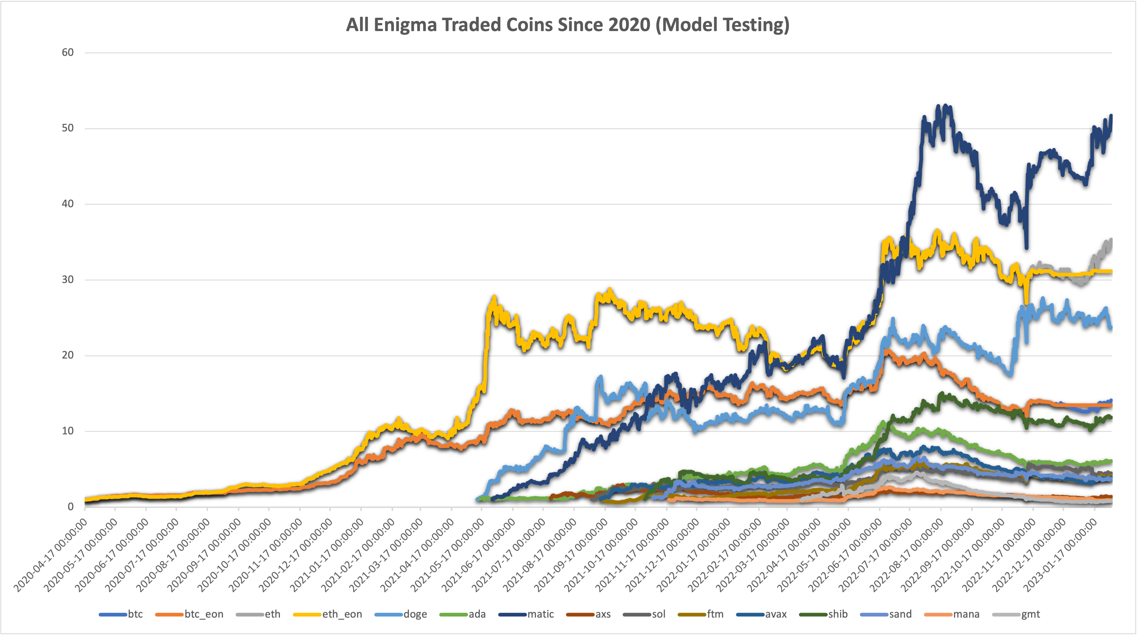
We attempt to find an optimal allocation that fulfills some given criteria from this data (DOT trading is omitted from the graph above because it makes everything else look small).

Naive Approach: Equal Weights

The most basic mix would be to weigh all tokens equally. Thus, each contract would get 1/14th of the portfolio. Important simplified assumptions:

1. We are ignoring that not all coins were available from the start, and give each coin 1/14th of the portfolio to trade with.

2. We are ignoring the fact that due to liquidity issues, not all coins could support trading volumes at all times.

The following profile emerges:

We will compare other mixes against this one.

Efficient Frontier

In MPT, we seek to construct a mix of assets, or trading pairs that sit along the efficient frontier. We can find this frontier by simulating thousands of possible portfolio weights (allocations) and then selecting those which maximize our preferred metric.

Implementing this, we construct 2 portfolios to:

1. Maximize Sharpe Ratio

2. Minimize Volatility

The full timeline is sliced into 11 intervals, with one new interval for each time we added a trading pair. The weights are calculated for each interval, such that we optimally allocate between available trading pairs. We also assume that all coins are trading 100% of the time.

At the end of each interval, we then take the cumulative returns and distribute them over the trading pairs of the next one, with the relevant weights. This assures that compounding remains in effect and we transition from one weighting to the next without disruption.

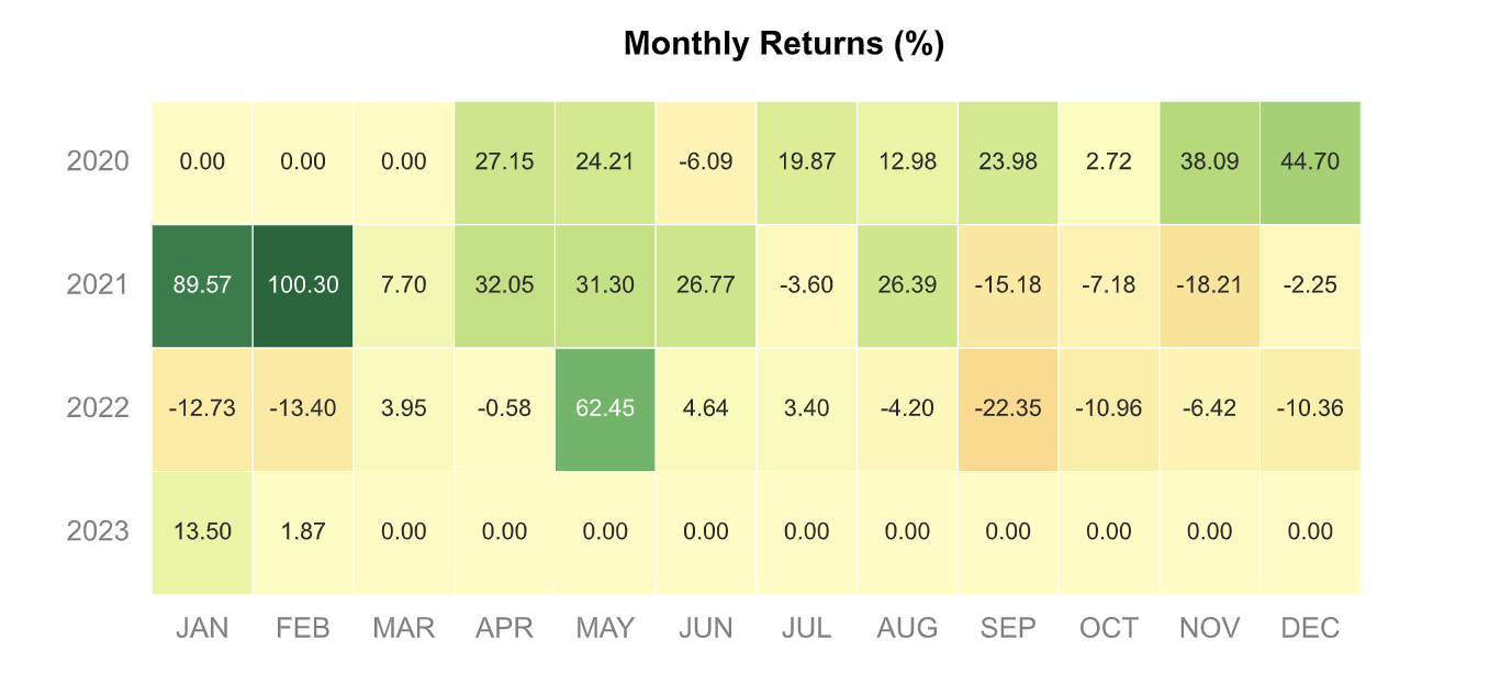
Minimizing Volatility

The first portfolio minimizes volatility. The following return profile emerges:

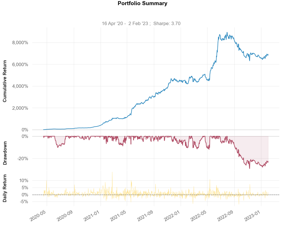
As we can see, our returns and Sharpe Ratio have more than doubled from our Naive approach. 6,905% return since inception, and a Sharpe Ratio of 3.7, our annualized volatility is 29%, and the Max Drawdown stands at -28%. Not bad.

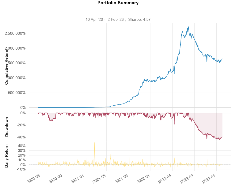
Maximizing Sharpe Ratio

The truly ridiculous portfolio emerges when we maximize for Sharpe. This leads to a height of over 2 million percent returns, likely due to the heavy weighting on DOT trading, which saw fantastical returns in our models, but would likely not be able to trade the amount of money required in this weighting. A more sophisticated analysis with more constraints should be run here to find a true estimate of what could realistically have been achieved.

Conclusion

As we can see from the simple analysis, portfolio optimization is an extremely powerful tool to maximize returns and minimize risk. We should devote a fair bit of effort to this.

Continued Research: Model Weighting

As mentioned above, we can conduct the same kind of analysis not between trading pairs in the aggregate, but between individual models within a trading pair. For example, it might be that some model timeframes perform better than others in certain periods. Rebalancing allocation to each model in an optimal way may lead to further improvements in the system.

A Look at Timeframes

It appears as though, on the whole, shorter timeframes have had slightly worse results than longer ones. A further breakdown under which market conditions, and during which periods shorter models performed better would be interesting. We can see from the below charts that Enigma does well between 45-minute, and 2-hour predictions. To what extent this performance is due to lower trade volume and therefore lower fees, is not known at the moment (We should look into cost per trade, which is not something that Binance data shows, but something we should calculate on our own end)

Optimizing BTC Model Allocation

Running a similar portfolio optimization as above, we first look at an equal allocation between all models. This allocation simply divides 1 by the number of models at the time and allocates according to that fraction.

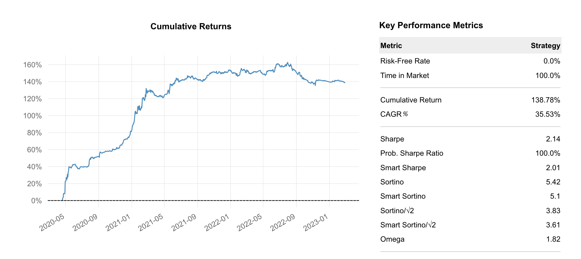
The Equal Weight allocation results in a 138.78% return with a Sharpe of 2.14.

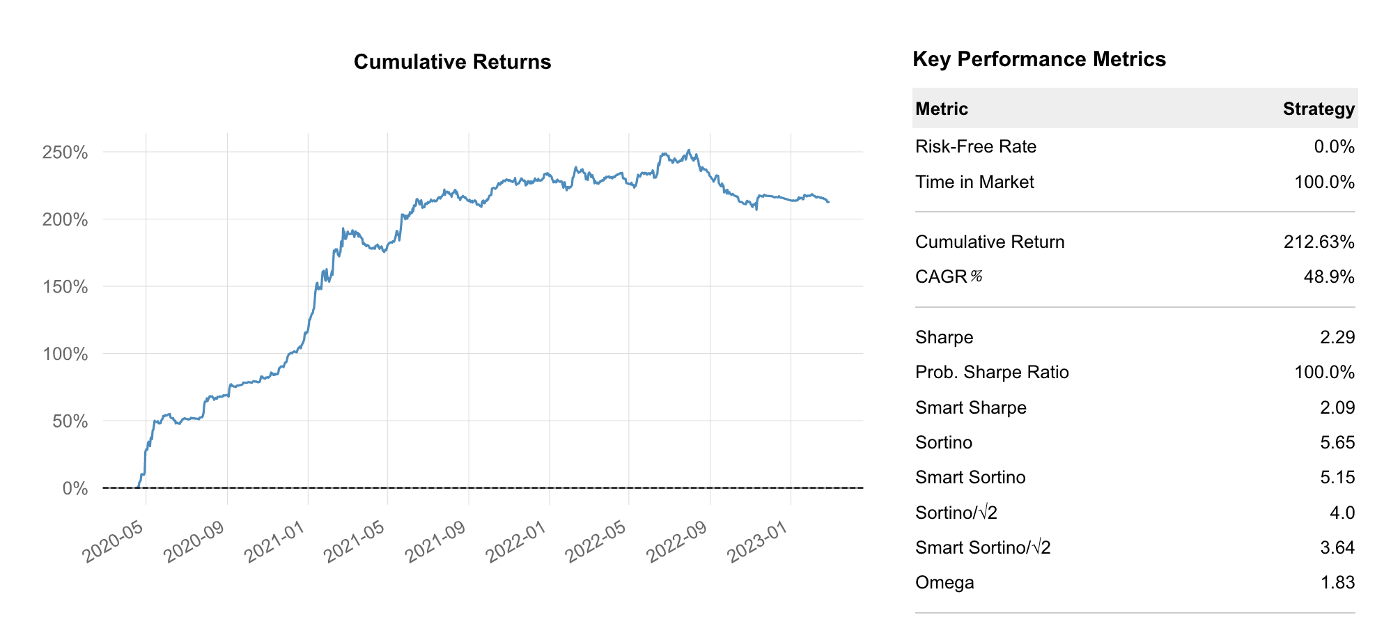
The Sharpe Ratio optimized allocation produces 212.63% over the same time and a Sharpe Ratio of 2.29. This is a 53% improvement over the Equal Weight allocation.

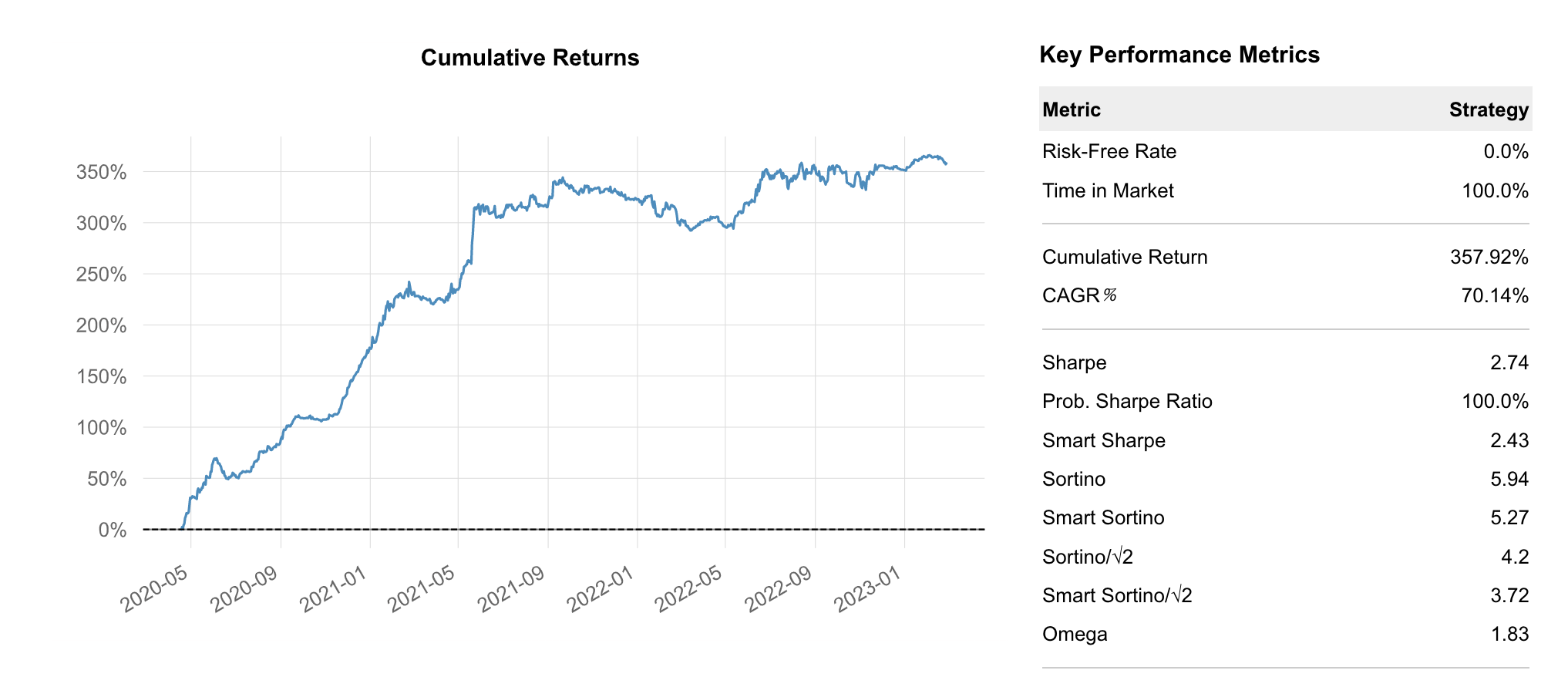
Optimizing ETH Model Allocation

Running the exact same analysis with ETH models, we can see the Equal Weight allocation returns 176.17% with a Sharpe of 2.42.

Using the Sharpe Optimized version, we achieve 357.92% with a Sharpe of 2.74. That is an incredible 103% improvement, simply by allocating between models more optimally.

*Development Note: the evaluation of models forward-fills models that are no longer in use. That means that theoretically, the weight allocation could allocate to models that no longer do anything and have zero returns. This is a by-product of my hasty code writing… In production, this should definitely be optimized as well. It affects the equal allocation more than the optimized one because in the optimized one, zero-change models would not get much weight assigned to them. They may still affect the risk metrics in negative months though when zero returns are better than negative returns. They mess up the calculation somewhat. I only noticed this problem later. *

F*urther note: the average of all models is treated like another model, so it receives a weight. This should not be the case. It would not make a huge difference, but it is still inaccurate. Will change. *