Documentation for Portfolio Optimization with XGBoost Classification

Source: Notion | Last edited: 2025-03-21 | ID: 1202d2dc-3ef...

---

Overview

This project explores capital allocation strategies for Profit and Losses (PnLs) using the XGBoost classification method. The core idea is to leverage XGBoost models to classify PnLs into two categories—going up or going down—and use the prediction probabilities to allocate capital accordingly. Specifically, we developed XGBoost classification models for each cryptocurrency. The GitHub repository is linked here.

The classification models are trained using historical PnL data. The allocation is generated based on prediction probabilities using a maximum-probability allocation strategy.

The main objective is to develop an efficient, prediction-based allocation strategy for cryptocurrencies, leveraging the classification capabilities of XGBoost to guide capital distribution. The key steps involved in the project and several versions of experiments are outlined as follows:

Exploratory Data Analysis (EDA)

In this project, several exploratory data analysis (EDA) techniques were applied to understand the behavior of the PnL data and to inform feature engineering for the models. Key findings from the EDA are summarized as follows:

1. PnL Fluctuations: Visualizations revealed that the PnLs are highly volatile, with fluctuations occurring every 1-3 hours across all cryptocurrencies. This suggests that short-window statistical features could be valuable.

2. PnL Statistics: The mean values of the PnLs were quite small—[0.000261, 0.000358, 0.000458, 0.000626]—while DOGE exhibited the highest volatility with a standard deviation [0.004255, 0.005531, 0.007200, 0.010724], making it the most fluctuating cryptocurrency among the four.

3. Correlation Analysis: The correlation matrix revealed the following relationships between the cryptocurrencies. The strong correlation indicates they could be used as features.

• BTC and ETH: Moderate correlation (corr = 0.61)
• ETH and ADA: Moderate correlation (corr = 0.52)
• DOGE: No significant correlation with any other cryptocurrency

1. Auto-Correlation: The auto-correlation plot indicated that lagging PnL values do not have strong predictive power. Therefore, traditional time series forecasting models like ARIMA may not be effective for this data.

2. Rolling Mean and Std Analysis: Rolling mean and rolling standard deviation were calculated with different window lengths (e.g., 1 week, 2 months). The results showed significant fluctuations in both the rolling mean and standard deviation, which decreased toward the latter part of the dataset,** indicating a potential data shift over time**.

3. Rolling Correlations: Rolling correlations fluctuated with a cycle length of approximately 1-2 months. This suggests that retraining the models with a 1-2 months rolling window could help capture the underlying data shifts more effectively.

4. Fluctuation Analysis: The analysis revealed that the PnLs changed direction nearly every time step, with an average fluctuation period of 2-time steps. Therefore, one simple idea is to construct a simple rolling mean, push it forward, and compare whether they are in the same direction. A simple rolling mean with a window of 2, shifted forward by 1-2 time steps, was explored and showed an accuracy of around 51.07%.

5. Cycle Detection: An analysis of positive vs. negative PnL counts for specific window lengths indicated cyclical fluctuations in the data. These fluctuations decreased toward the end of the data, further supporting the observation of a data drift.

6. Market Trend Signals: With the positive and negative counts, we can utilize these signals to construct market trend signals by comparing the present count values with a rolling mean count value. In these plot, we use the window to be 7*24 which is 1 week. We can see the market regime shift from these features. Then we should revise the train, validation, and test period so it includes several pattern of market regimes in each part.

Through this EDA, a gradual shift in the data was observed, particularly in the final 20% of the dataset. This shift coincided with a drop in model performance, suggesting that a sliding window training approach and refit predictions could help mitigate the impact of this drift.

Feature Engineering

Based on insights from the EDA, where the PnLs showed rapid fluctuations within 1-2 samples, short-window statistical features were identified as potentially valuable for capturing the data’s behavior. Therefore, I applied short-window techniques to the following features:

• Rolling statistics (Mean, Std)
• Differences and lags
• Rolling Min/Max values
• Cumulative sum of positive/negative moves
• Positive/Negative count ratios
• Momentum indicators
• Correlations
• DateTime features (Hour, Date, Week, Month, Day of the week, Weekend, Holiday)
• Grouped features (Difference of values compared to group medians)
• Going-Up specific features After testing various combinations of these features, it was observed that short-window features (with window sizes of 1 to 6) performed better than longer-window features (such as those using a 1-month window). Model performance declined when expanding the window size, aligning with the findings from the EDA that PnLs tend to shift rapidly every 1-3 samples.

The most effective feature set included:

• -rolling_windows: [2, 3, 4, 5, 6]
• -diff_windows: [1, 2, 3, 4, 5, 6]
• -lag_windows: [1, 2, 3, 4, 5, 6]
• -corr_windows: [168]
• -overall_market_trend_window: 168
• -crypto_market_trend_window: 168

Feature Selection

Two feature selection techniques were applied: Feature Importance (from XGBoost) and Boruta. It was observed that the Feature Importance method from XGBoost tended to lead to overfitting or less accurate models. In contrast, Boruta produced more reliable results. Consequently, Boruta was chosen for the final feature selection for these models.

Performance Metric

Upon reevaluating the problem, I concluded that Precision is the most suitable metric for this task. Since it is crucial to allocate investment only when the model is highly confident, prioritizing Precision ensures that capital is correctly allocated when the model predicts the ‘Going Up’ direction, thereby maximizing profitability. To further emphasize this, I implemented a custom Precision scorer with a higher weight on class 1 (Going Up), ensuring the model focuses more on accurate predictions for positive movements.

• -class_weight_0: 0.25
• -class_weight_1: 0.75
• -performance_metric: “custom_weighted_precision”

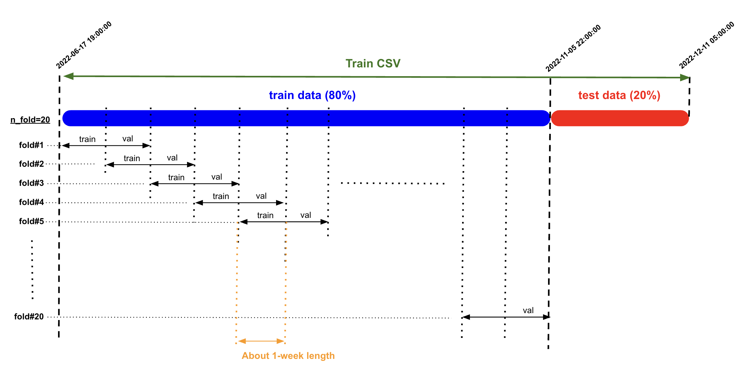
Model Training and Prediction

I experimented with different data-splitting methods for model training, including traditional cross-validation and sliding-window splitting. The sliding-window approach yielded better results, which is consistent with the EDA findings that the data shifts gradually over time.

For model prediction, I employed a refit prediction method, where the model is refitted using the last month of data before making each prediction. After testing different data lengths for refitting, I found that using 1-month windows provided the best results.

Retraining the model with longer historical data can reduce performance, as older data may not be as informative or relevant to the current market conditions. This is similar to trends observed in other markets, like crude oil (Brent/WTI), where using 2-3 years of historical data is optimal, while older data may become outdated and less useful. Similarly, in this case, shorter windows are more effective, as indicated by the EDA findings showing that PnLs fluctuate within 2-3 samples. Using shorter retraining windows can improve model performance by capturing the most relevant patterns.

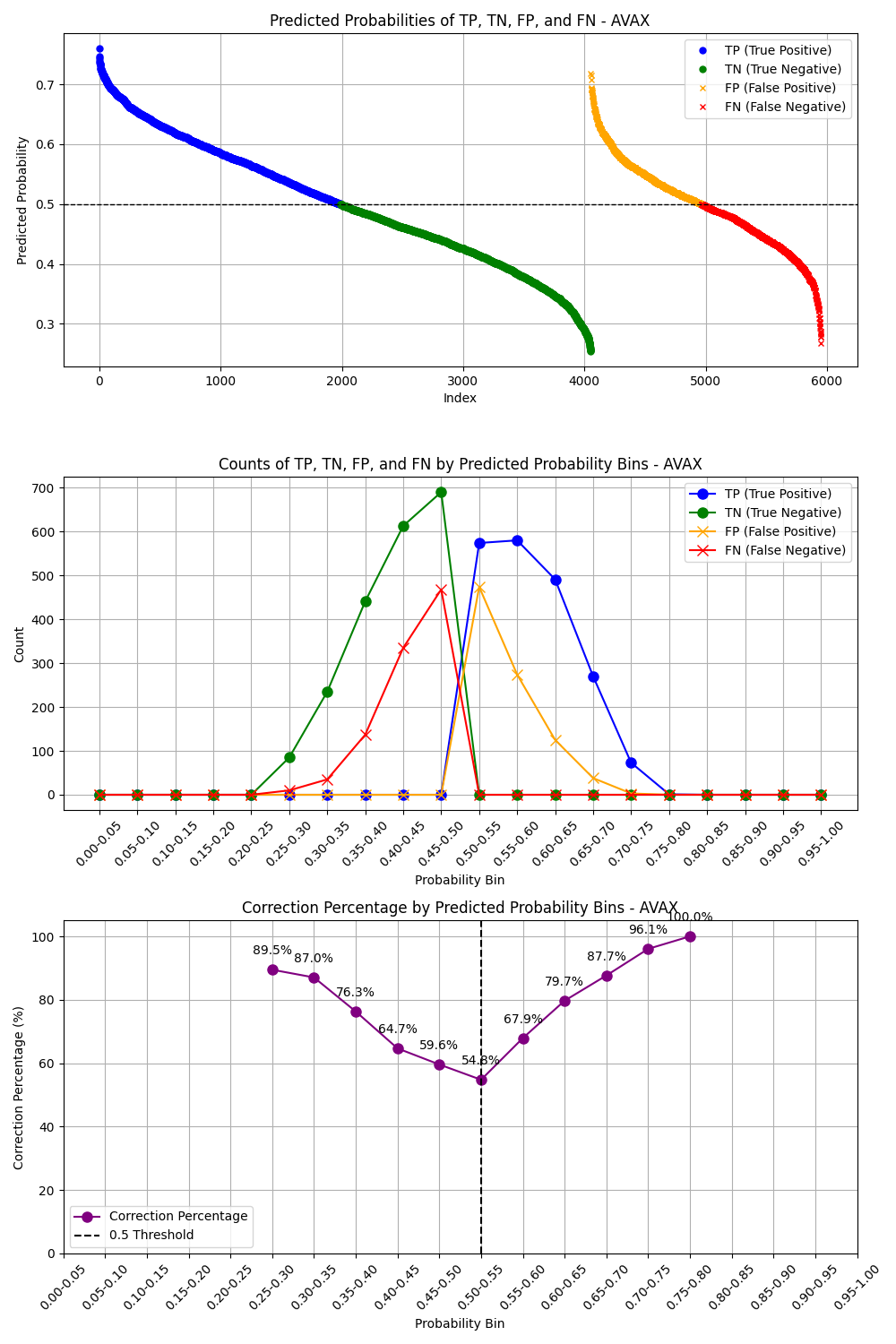
Model Training Results

After finishing model training, we have some plots to check the model performance. The first plot is to see the behavior of TP and TN whether it is more accurate when the probability is higher, this is the behavior of the prediction we want. The second plot is the confusion metrix.

**Train Data: **

Test Data:

After inspecting all plots, we can see that the precision scores are about 0.5-0.62

Allocation Strategy

Once the predictions were generated, I experimented several allocation strategies:

1. Positive Allocation: This strategy filters for ‘Going Up’ predictions and allocates capital to these PnLs based on the magnitude of their probabilities, provided they exceed a specified threshold.
2. Most Certain Allocation: This approach also filters for ‘Going Up’ predictions but allocates 100% of the capital to the PnL with the highest ‘Going Up’ probability (i.e., the most certain prediction).
3. Positive Allocation with Higher Threshold: This strategy is similar to the first, but with an increased threshold (0.6) to ensure that only the highest-confidence predictions receive an allocation.
4. Positive Allocation with Weighted Precision Score: In this strategy, we use the positive probabilities from prediction and also we construct 2 lookback values; lookback_interval and lookback_window. The strategy will check on every lookback_interval, gather data on the most recent lookback_window and calculate the precison score for each cryptocurrency, it then allocates to the time that the precision score above 0.5, otherwise, allocate zero.
5. Positive Allocation with Weighted Cumulative Return and Average PnL: In this strategy, we use the positive probabilities from prediction and also we construct 3 lookback values; lookback_interval, lookback_window, and lookback_avg_pnl. The strategy will check on every lookback_interval, gather data on the most recent lookback_window and calculate cumulative return and average pnl for each cryptocurrency, it then allocates to the time that the cumulative return and the average pnl is positive, otherwise, allocate zero.
   Among these, the **Positive Allocation with Weighted Cumulative Return and Average PnL **strategy yielded the highest cumulative return.

Best Result

With the chosen model and allocation strategy, the best result achieved a cumulative return of 2.19 on the validation_combined dataset. However it yields -17.78% MDD which is not good enough for production. The Risk-reward-Ratio is 6.69.

Key Observations

1. The Boruta feature selection method produced different sets of features each time the dataset was updated, which suggests that the model’s performance may vary over time. This indicates that it may be beneficial to periodically reselect features and retrain models using shorter training data windows.
2. Although Boruta outperformed Feature Importance, the initial random search with all features sometimes resulted in better-performing models than those using selected features. To further improve results, it may be worthwhile to explore other feature selection methods, such as MDA-Perturbation or Recursive Feature Elimination (RFE), or to refine the initial random search model by increasing the number of iterations.

Factor Analysis

One important insight we found is that the model performance varies by time, this align as we see the market regimes have been shifted from the market trend signals, therefore, finding good features from only train data may not be robust even we try to refit the model along the time. One idea is to check how much different of important features is changed by each data period; train, validation, test. Therefore, we calculate correlations of over 100,000 possible features to both target variable(continuous and discrete) and pick the top 50 features of each period to train the model.

We can some discrepancies of important features on different data periods. Several important features from Train period are not that important in Validation and Test period, same happened on Validation and Test period. This indicates that the market evolves over times. Therefore, using all combinations of these features might help capture change along the way.

Unfortunately, after training models with features from this factor analysis, we could not have a better result.

Running the Code (GitHub repository linked here.)

The repository is structured as follows:

Portfolio_Optimization_XGBC/
├── data/
│   ├── revised_train_combined_interval.csv
│   ├── revised_validation_combined_interval.csv
│   └── revised_test_combined_interval.csv
|-- eda/
|   ├── eda_and_dev.ipynb
|-- experiment/
|   ├── retraining_interval_and window/
|-- experiment_results/
|   ├── retraining_interval_and window/
|   |   ├── plots
|   |   ├── results
|-- factor_analysis_results/
|-- models/
|-- plot/
|   ├── train/
|   |   ├── confusion_matrix.png
|   |   ├── correction_plot.png
|   |   ├── returns_plot.png
|   ├── test/
|   |   ├── confusion_matrix.png
|   |   ├── correction_plot.png
|   |   ├── returns_plot.png
|   ├── eval/
|   |   ├── returns_plot.png
|-- refitting_parameters/
|-- results/
|-- selected_features/
|-- src/
|   ├── helpers/
|   |   ├── __init__.py
|   |   ├── analysis.py
|   |   ├── data.py
|   |   ├── factor_utils.py
|   |   ├── feature_engineering.py
|   |   ├── get_arguments.py
|   |   ├── mlflow_log.py
|   |   ├── model_training.py
|   |   ├── plot.py
|   |   └── strategy.py
|   ├── train.py
|   ├── eval.py
|   ├── factor_analysis.py
|   ├── train_fa_discrete.py
|   ├── eval_fa_dscrete.py

The historical PnL data used for both training and evaluating models is stored in the “data” folder. The “eda” folder contains Jupyter notebook files with important and useful exploratory data analysis results. The “models” folder stores the trained models, while the “selected_features” folder contains the selected features used for training and evaluation. The “refitting_parameters” stores the optimal refitting interval and window for each tranied model. The “plot” folder is organized into three subfolders (train/, test/, and eval/) to store the visualization outputs generated during different stages of the process, including confusion matrices, correlation plots, and returns plots. The “results” folder stores training and evaluation results. The “factor_analysis_results” stores the results of correlation analysis of the target variable with all possible features. “Finally, the “src” folder contains the core implementation, including two main scripts (train.py and eval.py) along with a helpers package containing utility modules for feature engineering, argument parsing, allocation prediction, and other supporting functions.

Usage

You can run the project in two ways: by using a Dev Container or by running it in your local Python environment.

Running in Dev Container

1. Clone the repository to your local machine:

git clone https://github.com/Eon-Labs/Portfolio_Optimization_XGBC.git

1. Open the repository in an IDE such as Cursor or VSCode and install the Dev Container extension.
2. Build and run the Dev Container using the “Reopen in Container” option from the command palette.
3. Run 5 following commands to train, evaluate, and analyze the XGB Classification models:

python -m src/train.py
python -m src/eval.py
python -m src/factor_analysis.py
python -m src/train_fa_discrete.py
python -m src/eval_fa_discrete.py

Please note that the training process will take about 8 hours to finish while the evaluation process will take about 2 hours. The factor analysis needs to be run saparately by each data interval, it takes about one hour each interval.

Running in Local Python Environment

1. Clone the repository to your local machine:

git clone https://github.com/Eon-Labs/Portfolio_Optimization_XGBC.git

1. Navigate to the repository and create a new conda environment:

conda create -n el_ca_xgbc python=3.10
conda activate el_ca_xgbc

1. Install the required dependencies:

pip install -r requirements.txt

1. Run 5 following commands to train, evaluate, and analyze the XGB Classification models:

python -m src/train.py
python -m src/eval.py
python -m src/factor_analysis.py
python -m src/train_fa_discrete.py
python -m src/eval_fa_discrete.py

Please note that the training process will take about 8 hours to finish while the evaluation process will take about 2 hours. The factor analysis needs to be run saparately by each data interval, it takes about one hour each interval.

To run the commands

There are 5 commands to run to train, evaluate, and analyze the model

1. python -m src/train.py
2. python -m src/eval.py
3. python -m src/factor_analysis.py
4. python -m src/train_fa_discrete.py
5. python -m src/eval_fa_discrete.py

1. Train the XGB Classification Models

To train the XGB Classification models using the historical PnLs data, run the following command:

python -m src/train.py

The code will pull the historical PnL data as specified in the argument to train the models.

There are a number of parameters for the training process which you can change for your experiment. The training parameters along with their default values include:

• -mlflow_server: “local”
• -experiment_name: “XGBC Capital Allocation”
• -run_name: “xgbc_individual_models”
• -train_data_path: “data/revised_train_combined_interval.csv”
• -warmup_data_path: “data/revised_train_combined_interval.csv”
• -eval_data_path: “data/revised_validation_combined_interval.csv”
• -cryptos: [“BTC”, “ETH”, “ADA”, “DOGE”, “SOL”, “SHIB”, “AVAX”, “DOT”, ]
• -data_interval: “1h”
• -prediction_interval: 4
• -class_weight_0: 0.25
• -class_weight_1: 0.75
• -performance_metric: “custom_weighted_precision”
• -rolling_windows: [2, 3, 4, 5, 6]
• -diff_windows: [1, 2, 3, 4, 5, 6]
• -lag_windows: [1, 2, 3, 4, 5, 6]
• -corr_windows: [168]
• -overall_market_trend_window: 168
• -crypto_market_trend_window: 168
• -feature_selection_method: “boruta”
• -retraining_interval: 6
• -retraining_window: 168
• -test_size: 0.2
• -cv_folds: 20
• -n_iters_random_search_all_features: 15
• -n_iters_random_search_selected_features: 100
• -n_estimators_max: 1000
• -max_depth_max: 10
• -learning_rate_max: 0.5
• -reg_lambda_max: 2000
• -retraining_interval_lists: [4, 8, 12, 16, 20, 24, 36]
• -retraining_window_lists: [ 7 * 24, 2 * 7 * 24, 4 * 7 * 24, 2 * 4 * 7 * 24, 3 * 4 * 7 * 24, ]
• -lookback_intervals: [ 1, 2, 4, 6, 8, 12, 16, 20, 24, 36, 72, ]
• -lookback_windows: [ 3, 6, 9, 12, 24, 36, 48, 72, 96, 144, 7 * 24, 2 * 7 * 24, 3 * 7 * 24, 4 * 7 * 24, ]
• -lookback_avg_pnl_windows: [ 3, 4, 6, 8, 12, 16, 24, 2 * 24, 3 * 24, 7 * 24, 4 * 7 * 24, 2 * 4 * 7 * 24, 3 * 4 * 7 * 24, ]
• -optimal_lookback_interval: 1
• -optimal_lookback_window: 336
• -optimal_lookback_avg_pnl_window: 12
• -no_rolling_cryptos: [ “BTC”, “DOGE”, “SOL”, “AVAX”, ]
• -rolling_cryptos: [ “ETH”, “ADA”, “SHIB”, “DOT”, ] For example, you can run this following command to train the models with 5 iterations of all features random search and 100 iterations of selected features random search with logging to EonLabs MLflow server:

python -m src/train.py --mlflow_server "eonlabs" --run_name "xgbc_niter_5_100" --n_iters_random_search_all_features 5 --n_iters_random_search_selected_features 100

The code will automatically save the trained XGBC models as “trained_{cryptocurrency}_model.joblib” in the “models” folder. These trained models will be used for the evaluation process.

Please note that the training process may take about 8 hours to finish.

2. Evaluate the XGB Classification Models

To evaluate the XGB Classification models, run the following command:

python -m src/eval.py

The code will use the historical PnL data as specified in the argument to evaluate the model performance.

There are some parameters for the evaluation process which you can change for your experiment. The evaluation parameters along with their default values include:

• -warmup_data_path: “data/revised_train_combined_interval.csv”
• -eval_data_path: “data/revised_validation_combined_interval.csv”
• -optimal_lookback_interval: 1
• -optimal_lookback_window: 336
• -optimal_lookback_avg_pnl_window: 12
• -no_rolling_cryptos: [ “BTC”, “DOGE”, “SOL”, “AVAX”, ]
• -rolling_cryptos: [ “ETH”, “ADA”, “SHIB”, “DOT”, ] The optimal lookback interval, window, and avg_pnl_window is showed when running training the model, the no_rolling_cryptos and rolling_cryptos come from checking the best model performance in training process. If you retrain the model, check these values and set it for the evaluation.

For example, you can run this following command to evaluate the model performance of “data/revised_test_combined_interval.csv” with the “data/revised_validation_combined_interval.csv” as a warmup file, along with logging to EonLabs MLflow server and the run name is “xgbc_niter_5_100”:

python -m src/eval.py --mlflow_server "eonlabs" --run_name "xgbc_niter_5_100" --eval_data_path "data/revised_test_combined_interval.csv" --warmup_data_path "data/revised_validation_combined_interval.csv"

Please note that the training process may take about 2-4 hours to finish.

3. Run Factor Analysis

To run the correlation analysis for all possible features to the target valriable(the future compound pnl), run the following command:

python -m src/factor_analysis.py

There are some parameters for the analysis which you can change for your experiment. The default parameters include:

• -train_data_path: “data/revised_train_combined_interval.csv”
• -validation_data_path: “data/revised_validation_combined_interval.csv”
• -test_data_path: “data/revised_test_combined_interval.csv”
• -cryptos: [“BTC”, “ETH”, “ADA”, “DOGE”, “SOL”, “SHIB”, “AVAX”, “DOT”, ]
• -data_interval: “1h”
• -prediction_interval: 4
• -data_period: “train”
• -targte_type: “discrete”
• -rolling_windows: [ 2, 3, 4, 5, 6, 12, 24, 2 * 24, 3 * 24, 7 * 24, 2 * 7 * 24, 4 * 7 * 24, 504, 1440, 2160, ]
• -diff_windows: [ 1, 2, 3, 4, 5, 6, 7, 8, 9, 10, 11, 12, 24, 2 * 24, 3 * 24, 7 * 24, ]
• -lag_windows: [ 1, 2, 3, 4, 5, 6, 7, 8, 9, 10, 11, 12, 24, 2 * 24, 3 * 24, 7 * 24, ]
• -corr_windows: [ 24, 3 * 24, 7 * 24, 2 * 7 * 24, 4 * 7 * 24, 2 * 4 * 7 * 24, 3 * 4 * 7 * 24, ]
• -overall_market_trend_window: [24, 3 * 24, 7 * 24, 4 * 7 * 24]
• -crypto_market_trend_window: [24, 3 * 24, 7 * 24, 4 * 7 * 24]
• -technical_windows: [24, 3 * 24, 7 * 24, 4 * 7 * 24] You can speficy type of the target as discrete or continuous. Also, due to insufficient memory usage, we need to run it 3 times by changing the data_period for all “train”, “val”, and “test”. Then, the result will be stored in factor_analysis_results folder. The top correlated features will be stores in selected_features folder with the name of {crypto}fa{target_type}_selected_feature_names.joblib.

For example, you can run this following command toanalyze the discrete target pnl on the validation dataset:

python -m src/factor_analysis.py --targte_type "discrete" --data_period "val"

4. Train XGB Models with variables from factor analysis

After running the factor analysis, we can train the model using top correlated features from the analysis as:

python -m src/train_fa_discrete.py

There are a number of parameters for the training process which you can change for your experiment. The training parameters along with their default values include:

• -mlflow_server: “local”
• -experiment_name: “XGBC Capital Allocation”
• -run_name: “xgbc_individual_models”
• -train_data_path: “data/revised_train_combined_interval.csv”
• -warmup_data_path: “data/revised_train_combined_interval.csv”
• -eval_data_path: “data/revised_validation_combined_interval.csv”
• -cryptos: [“BTC”, “ETH”, “ADA”, “DOGE”, “SOL”, “SHIB”, “AVAX”, “DOT”, ]
• -data_interval: “1h”
• -prediction_interval: 4
• -class_weight_0: 0.25
• -class_weight_1: 0.75
• -performance_metric: “custom_weighted_precision”
• -rolling_windows: [ 2, 3, 4, 5, 6, 12, 24, 2 * 24, 3 * 24, 7 * 24, 2 * 7 * 24, 4 * 7 * 24, 504, 1440, 2160, ]
• -diff_windows: [ 1, 2, 3, 4, 5, 6, 7, 8, 9, 10, 11, 12, 24, 2 * 24, 3 * 24, 7 * 24, ]
• -lag_windows: [ 1, 2, 3, 4, 5, 6, 7, 8, 9, 10, 11, 12, 24, 2 * 24, 3 * 24, 7 * 24, ]
• -corr_windows: [ 24, 3 * 24, 7 * 24, 2 * 7 * 24, 4 * 7 * 24, 2 * 4 * 7 * 24, 3 * 4 * 7 * 24, ]
• -overall_market_trend_window: [24, 3 * 24, 7 * 24, 4 * 7 * 24]
• -crypto_market_trend_window: [24, 3 * 24, 7 * 24, 4 * 7 * 24]
• -technical_windows: [24, 3 * 24, 7 * 24, 4 * 7 * 24]
• -feature_selection_method: “boruta”
• -retraining_interval: 6
• -retraining_window: 168
• -test_size: 0.2
• -cv_folds: 20
• -n_iters_random_search_all_features: 15
• -n_iters_random_search_selected_features: 100
• -n_estimators_max: 1000
• -max_depth_max: 10
• -learning_rate_max: 0.5
• -reg_lambda_max: 2000
• -retraining_interval_lists: [4, 8, 12, 16, 20, 24, 36]
• -retraining_window_lists: [ 7 * 24, 2 * 7 * 24, 4 * 7 * 24, 2 * 4 * 7 * 24, 3 * 4 * 7 * 24, ]
• -lookback_intervals: [ 1, 2, 4, 6, 8, 12, 16, 20, 24, 36, 72, ]
• -lookback_windows: [ 3, 6, 9, 12, 24, 36, 48, 72, 96, 144, 7 * 24, 2 * 7 * 24, 3 * 7 * 24, 4 * 7 * 24, ]
• -lookback_avg_pnl_windows: [ 3, 4, 6, 8, 12, 16, 24, 2 * 24, 3 * 24, 7 * 24, 4 * 7 * 24, 2 * 4 * 7 * 24, 3 * 4 * 7 * 24, ]
• -optimal_lookback_interval: 1
• -optimal_lookback_window: 12
• -optimal_lookback_avg_pnl_window: 16
• -no_rolling_cryptos: [“XXX”]
• -rolling_cryptos: [ “BTC”, “ETH”, “ADA”, “DOGE”, “SOL”, “SHIB”, “AVAX”, “DOT”, ] For example, you can run this following command to train the models with 5 iterations of all features random search and 100 iterations of selected features random search with logging to EonLabs MLflow server:

python -m src/train_fa_discrete.py --mlflow_server "eonlabs" --run_name "xgbc_niter_5_100" --n_iters_random_search_all_features 5 --n_iters_random_search_selected_features 100

The code will automatically save the trained XGBC models as “discrete_trained_{cryptocurrency}_model.joblib” in the “models” folder. These trained models will be used for the evaluation process.

Please note that the training process may take about 8 hours to finish.

5. Evaluate XGB Models with variables from factor analysis

After training the model using top correlated features from the analysis, we can evaluate the result as:

python -m src/eval_fa_discrete.py

There are some parameters for the evaluation process which you can change for your experiment. The evaluation parameters along with their default values include:

• -warmup_data_path: “data/revised_train_combined_interval.csv”
• -eval_data_path: “data/revised_validation_combined_interval.csv”
• -optimal_lookback_interval: 1
• -optimal_lookback_window: 12
• -optimal_lookback_avg_pnl_window: 16
• -no_rolling_cryptos: [“XXX”]
• -rolling_cryptos: [ “BTC”, “ETH”, “ADA”, “DOGE”, “SOL”, “SHIB”, “AVAX”, “DOT”, ] The optimal lookback interval, window, and avg_pnl_window is showed when running training the model, the no_rolling_cryptos and rolling_cryptos come from checking the best model performance in training process. If you retrain the model, check these values and set it for the evaluation.

For example, you can run this following command to evaluate the model performance of “data/revised_test_combined_interval.csv” with the “data/revised_validation_combined_interval.csv” as a warmup file, along with logging to EonLabs MLflow server and the run name is “xgbc_niter_5_100”:

python -m src/eval.py --mlflow_server "eonlabs" --run_name "xgbc_niter_5_100" --eval_data_path "data/revised_test_combined_interval.csv" --warmup_data_path "data/revised_validation_combined_interval.csv"

Additional: Retraining Interval and Window Experiments

This experiment tests different combinations of retraining intervals and windows to find optimal values for model performance. The process involves two steps:

1. Run the experiments and collect results:

python -m experiment.retraining_interval_and_window.retraining_interval_and_window_exp

This will execute evaluation processes with different combinations of retraining intervals and windows, saving results to experiment_results/retraining_interval_and_window/results/retraining_interval_and_window_results.csv.

You can customize the intervals and windows to test using command line arguments:

• -retraining_interval: List of retraining intervals in hours
• -retraining_window: List of retraining windows in hours For example:

# Test single interval and window combination
python -m experiment.retraining_interval_and_window.retraining_interval_and_window_exp --retraining_interval 24 --retraining_window 168

# Test multiple intervals with single window
python -m experiment.retraining_interval_and_window.retraining_interval_and_window_exp --retraining_interval 24 48 72 --retraining_window 168

If no intervals or windows are specified, the experiment will use default values:

• Intervals: 6M, 3M, 2M (in hours)
• Windows: 1M, 2M, 3M (in hours)

1. Generate visualization plots:

python -m experiment.retraining_interval_and_window.retraining_interval_and_window_plot

This will create various plots to analyze the results, including:

• Heatmaps showing relationships between intervals, windows, and metrics
• Window comparison line plots
• 3D surface plots All plots will be saved in experiment_results/retraining_interval_and_window/plots/.

The experiment collects several performance metrics:

• Cumulative Return
• Maximum Drawdown
• Sharpe Ratio
• Calmar Ratio
• Penalized versions of each metric Please note that running the complete experiment suite may take several hours depending on the number of combinations tested.